Inventing Curve AMM math

09 Oct, 2024

In this post, we'll invent Curve AMM math as if for the first time.

Here's the problem Curve wants to solve: how can we enable token trades [1] at a constant exchange rate [2] with almost no slippage?

For example, a trader wants to convert arbitrary amounts of USDC into DAI at the price of 1 USDC for 1 DAI.

Consider a liquidity pool containing 1,000 USDC and 1,000 DAI, for which trades must satisfy the Constant Sum invariant (CS):

$x+y=D$

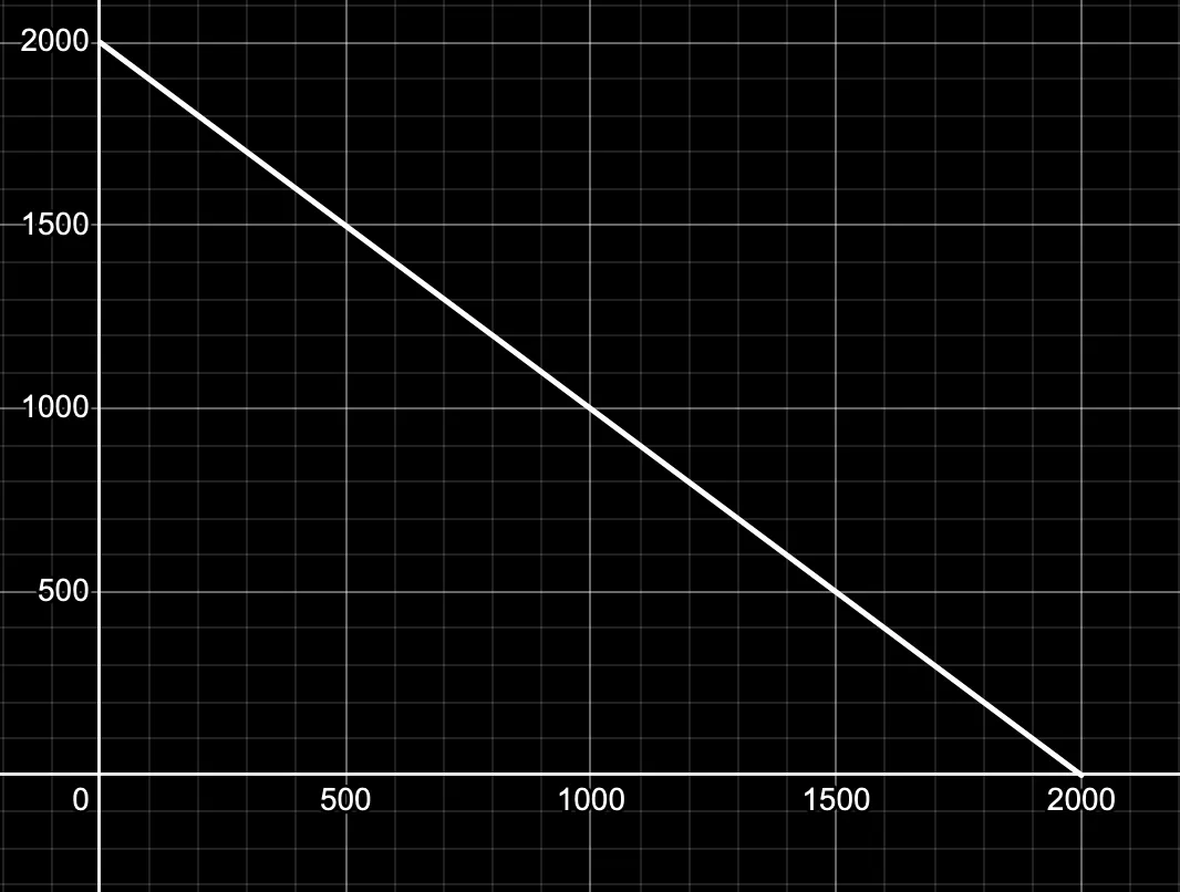
G.1: graph of the Constant Sum invariant with $(x+y)=D=2000$

We'll use $x$ to represent the total USDC tokens in the pool and $y$ to represent the total DAI tokens in the pool.

All trades in the pool must satisfy CS which means the sum of all tokens in the pool after a trade $(x+dx)+(y-dy)$ must remain the same as the sum before the trade $x+y$.

$x+y=(x+dx)+(y-dy)$

$dy=dx$

So, we always get 1 DAI out of the pool in exchange for adding 1 USDC to the pool, and vice-versa. Although this gives us zero slippage on trades, this also means the pool can run out of tokens. For instance, you can buy up all of the 1,000 USDC in the pool for 1,000 DAI.

Pools in UniswapV2 don't suffer from this problem of running out of tokens because trades in those pools must satisfy the Constant Product invariant (CP):

$x*y=k$

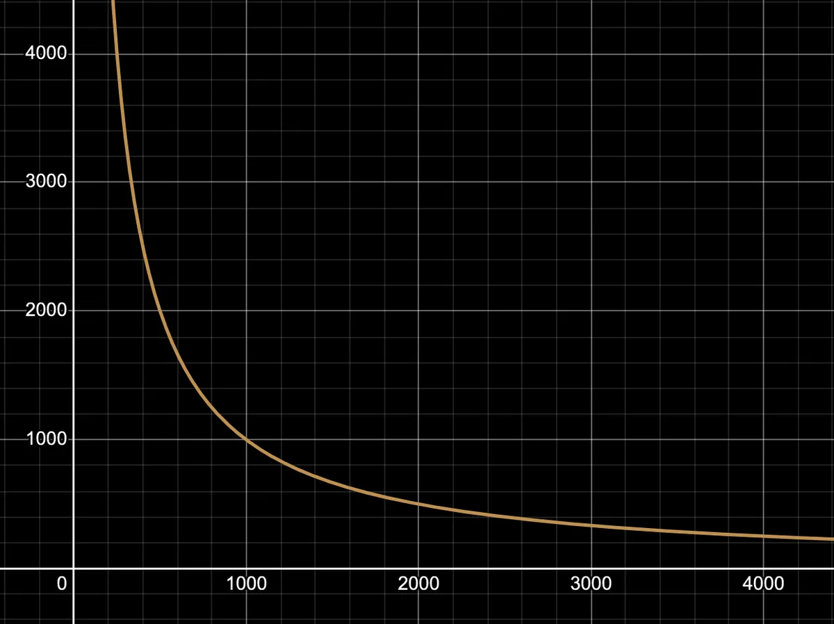
G.2: graph of the Constant Product invariant with $(x*y)=D=2000$

Consider the same liquidity pool containing 1,000 USDC and 1,000 DAI, for which trades must now satisfy CP. This means the product of the supply of both tokens in the pool after the trade must remain the same as before the trade.

$(x+dx)(y-dy)=xy$

$xy-xdy+ydx-dydx=xy$

$dy=\frac{y·dx}{x+dx}$

Now we cannot drain all of the pool's 1,000 DAI in exchange for 1,000 USDC. Adding 1,000 USDC ($dx=1000$) to the pool yields only 500 DAI ($dy=500$) out. Adding another 1,000 USDC returns only ~166.67 DAI.

The pool will never run out of DAI because the price of DAI in terms of USDC keeps increasing.

Although CP creates infinite liquidity for trades, it creates great slippage in trades (i.e. large deviations from the constant price at which we'd like to trade tokens such as USDC and DAI).

The ideal invariant for our pool would give the best of both worlds:

1. Constant exchange rate when the pool is fairly balanced (i.e. around 1:1 supply ratio of tokens in the pool)
2. Slippage as the pool becomes imbalanced, creating infinite liquidity for trades.

The graph of this ideal invariant would, therefore, look something like this:

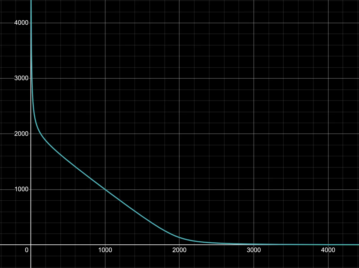
G.3: graph of the ideal invariant which is like CS in the center and CP at the axes

The graph is perfectly flat at its center where the pool is perfectly balanced at $x=y=1000$. It is largely flat around the center and only curves sharply near the axes where the pool is imbalanced, to create infinite liquidity.

In the remainder of the post, we'll come up with the invariant for this graph.

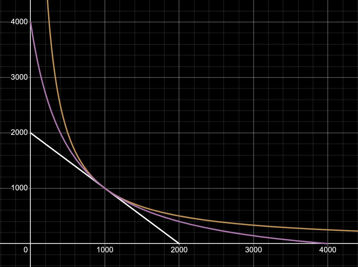
Let's look at the Constant Sum CS and Constant Product CP invariants again.

$x+y=D$

$x.y=(D/2{)}^2$

Here, $D$ stands for the total number of tokens in the pool when they have equal price. For example, $D=2000$ for a pool with 1,000 USDC and 1,000 DAI. The CP and CS curves intersect at this point where the pool is perfectly balanced.

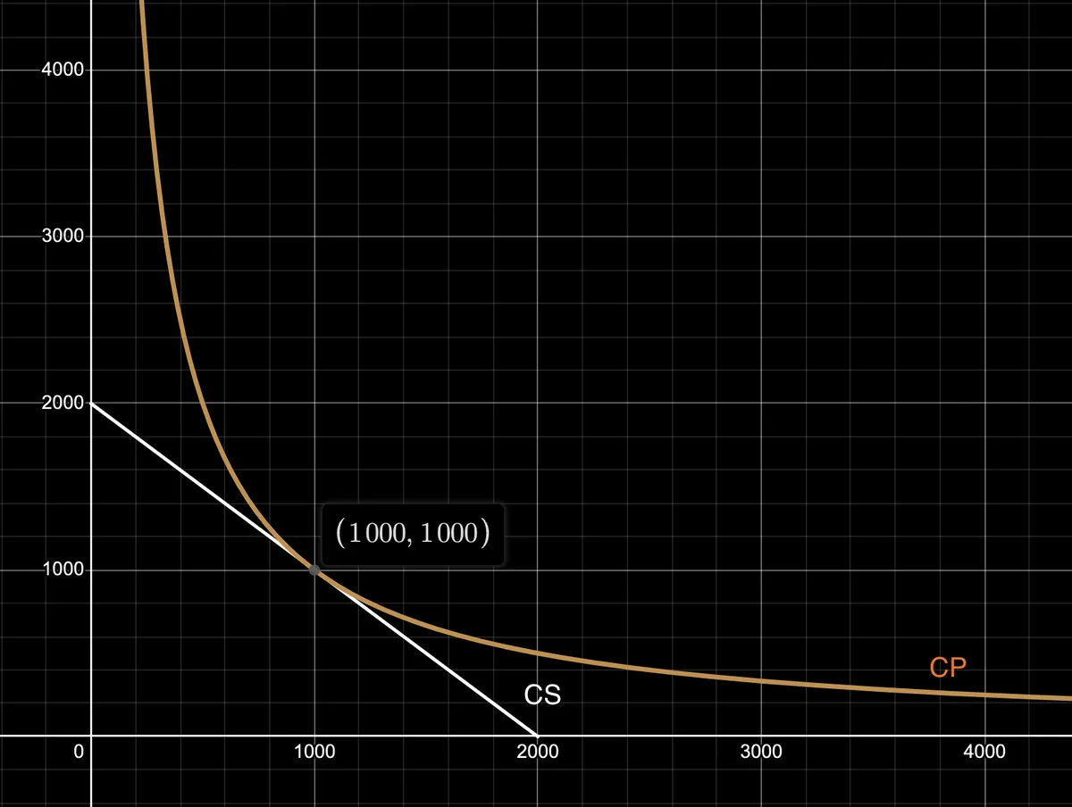
G.4: graph of the CS and CP together with $D=2000$

We're looking for a curve that sits right between the CP and CS curves. As we've noted, ideally our curve overlaps the CS curve almost exactly from the center out until near the axes where it would begin deviating asymptotically like the CP curve.

Let's start with an invariant that will guarantee a curve between CS and CP, and then modify this invariant.

Invariant v1

$(x+y)+x.y=D+(D/2{)}^2$

The v1 invariant simply adds the CS and CP invariants. We can verify algebraically that this invariant guarantees a curve between CS and CP.

Assume some $(a,b)\in CP$ or the region above the curve. So, $a.b\ge (D/2{)}^2$ and $a+b>D$. Therefore, $(a,b)$ doesn't satisfy the v1 invariant since

$(a+b)+a.b>D+(D/2{)}^2$

Now assume some $(p,q)\in CS$ or the region below the curve. So, $p.q<(D/2{)}^2$ and $p+q\le D$. Therefore, $(p,q)$ doesn't satisfy the v1 invariant since

$(p+q)+p.q<D+(D/2{)}^2$

Therefore, only points in the region between the CS and CP curves can possibly satisfy the v1 invariant.

Note that the point where the pool is perfectly balanced lies on both CS and CP and does satisfy the v1 invariant.

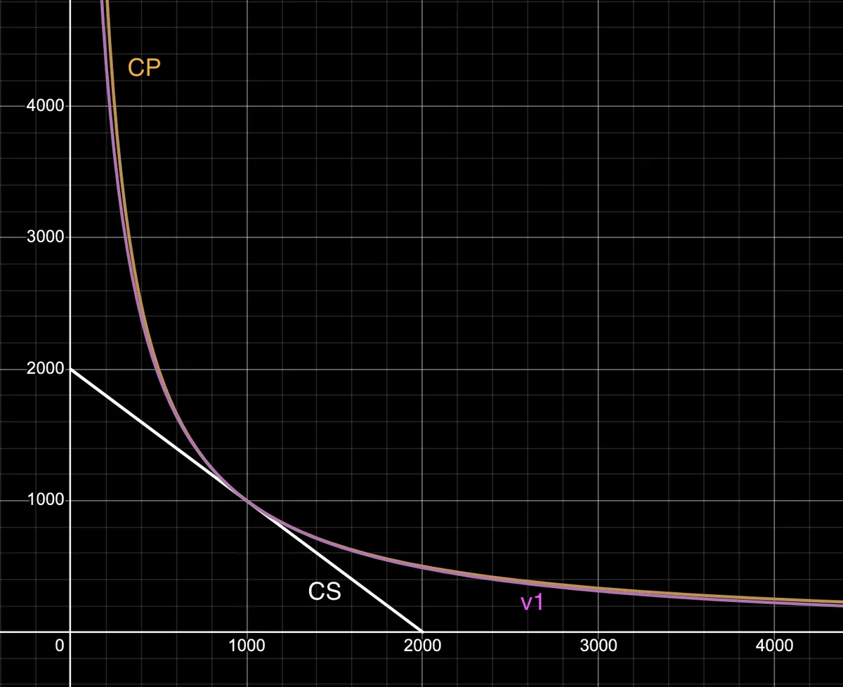
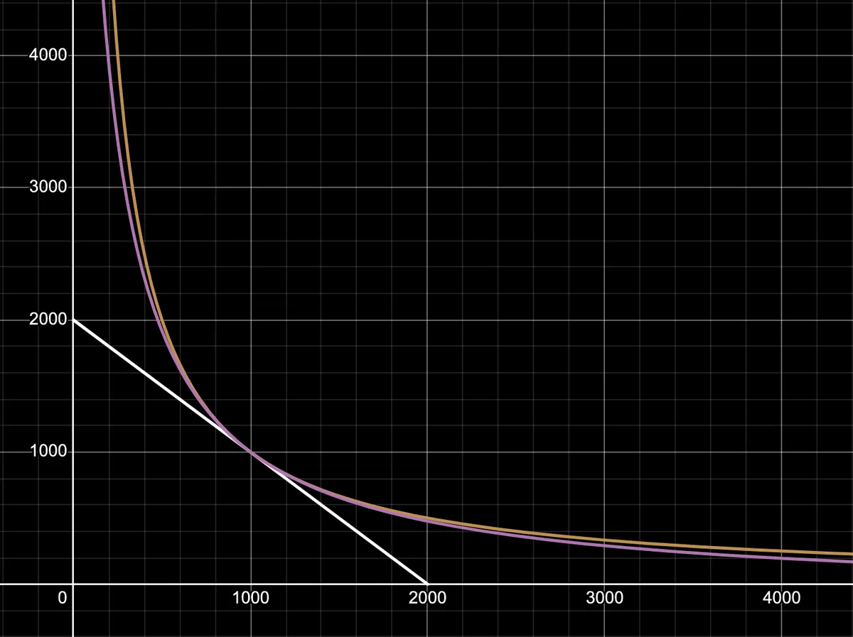
G.5: graph of the v1 invariant

The v1 invariant does not achieve what we set out to do - create a curve that is flat like CS in the middle and curves like CP near the axes. Currently, it closely tracks CP.

At a high level, we can expect this since the v1 invariant simply adds CS and CP and the multiplicative nature of CP is dominant over the additive nature of CS.

However, this is also the clue for how we should modify our invariant.

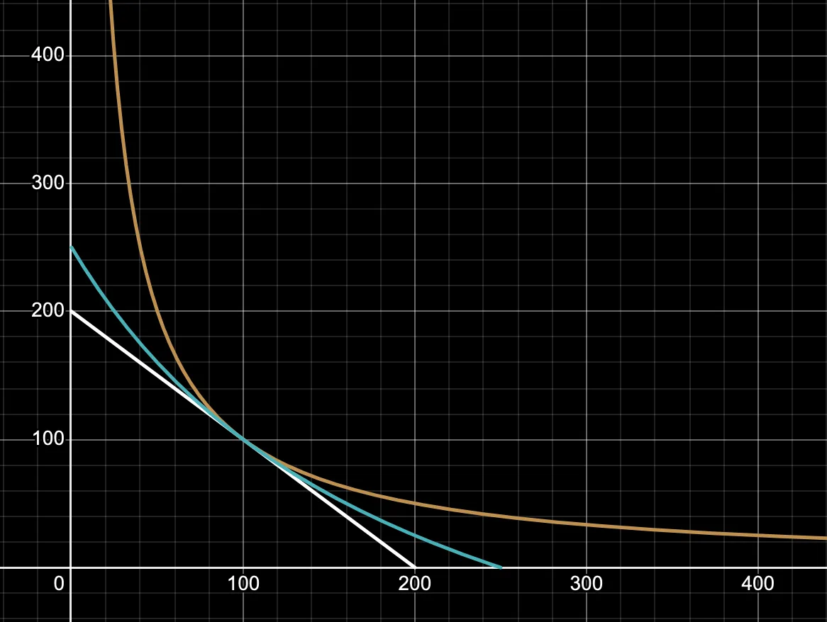
Invariant v2:

$\chi .(x+y)+x.y=\chi .D+(D/2{)}^2$

In the v2 invariant, we multiply the CS part by some positive factor $\chi$ to control the dominance of the CS part over the CP part. In other words, $\chi$ controls the flatness of the curve.

G.6: graph of the v2 invariant with $\chi =100$

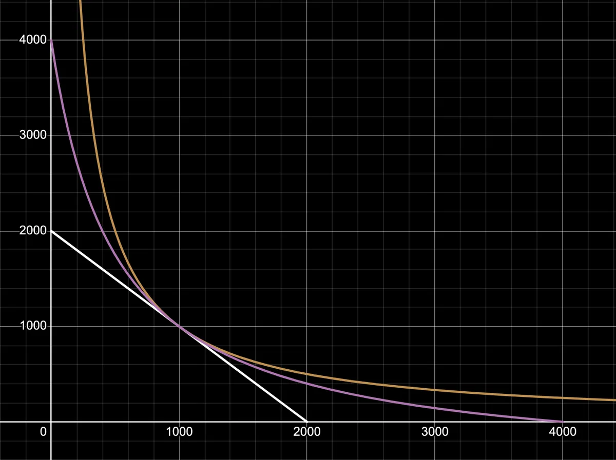
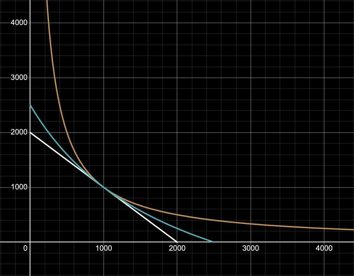
G.7: graph of the v2 invariant with $\chi =500$

As $\chi \to \infty$ the curve approaches CS and as $\chi \to 0$ the curve approaches CP. We can re-arrange the v2 invariant equation to concretely see why:

Let $c>0$

$(\chi +c).(x+y)+x.y=(\chi .D)+(D\backslash 2{)}^2$

$\chi .(x+y)+x.y=\chi .D+(D/2{)}^2+c(D-(x+y))$

We know $c(D-(x+y))$ is some negative quantity since $x+y>D$ for all $(x,y)$ above CS. So, increasing the value of $\chi$ has led to the same v2 invariant except with a smaller R.H.S. This means the L.H.S. must also become smaller for the invariant to be satisfied.

Therefore, for any fixed value of $x$, the corresponding value of $y$ becomes smaller when we increase $\chi$, and so, the curve flattens.

At this point, the factor $\chi$ affects the flatness of our curve differently for different pool sizes i.e. different values of $D$.

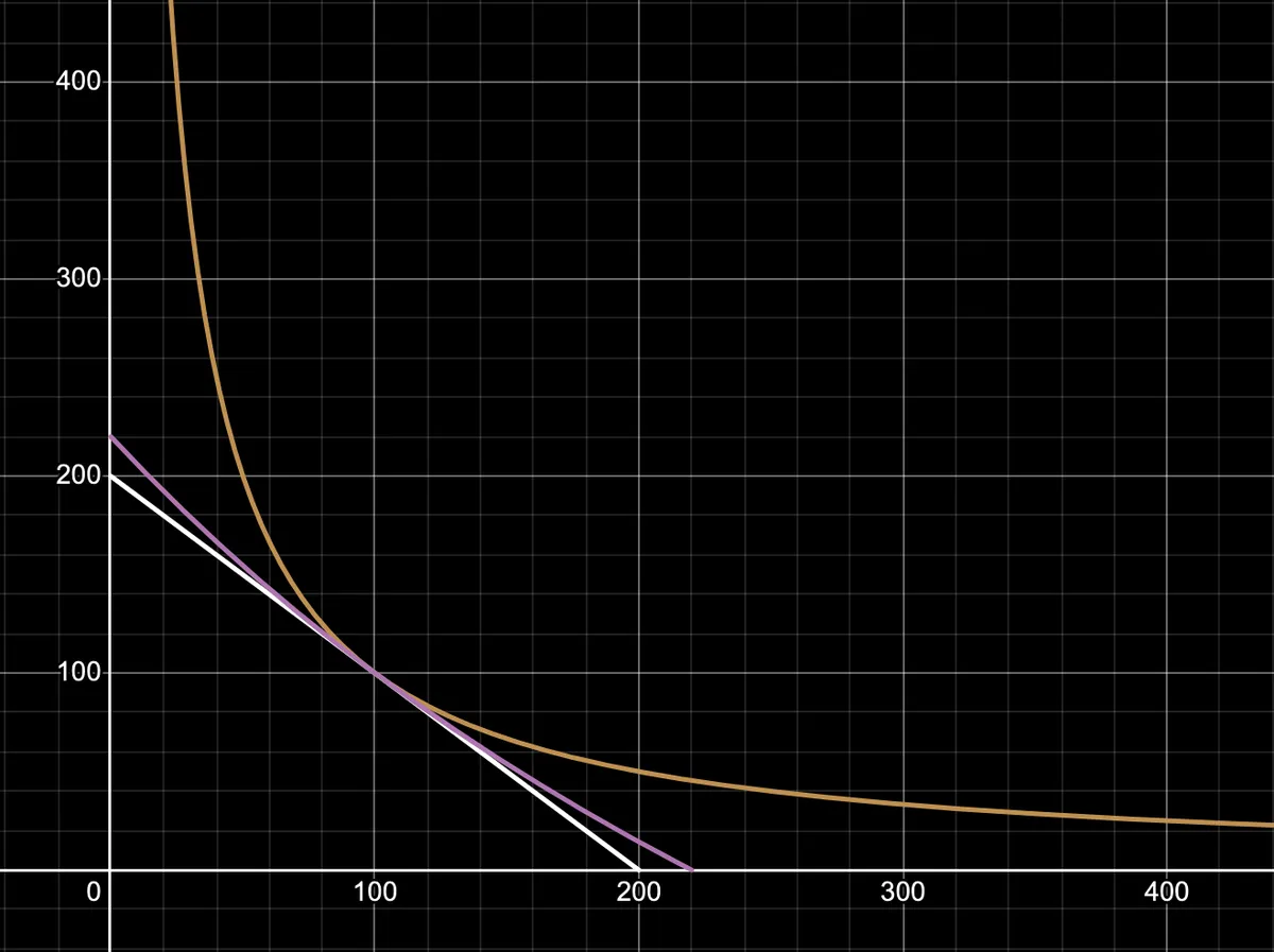
G.8: graph of the v2 invariant with $\chi =500$ and $D=200$

G.9: graph of the v2 invariant with $\chi =500$ and $D=2000$

Therefore, e.g. $\chi =10$ by itself does not communicate anything meaningful about the flatness of the curve, since the overall effect of $\chi$ depends on the size of the pool in consideration.

Invariant v3:

$\chi D.(x+y)+x.y=\chi .D^2+(D/2{)}^2$

In the updated v3 invariant, we multiply $\chi$ with the size of the pool $D$. Now, e.g. $\chi =10$ communicates the same level of flatness of the invariant curve for a pool of any size. We can verify this algebraically by re-arranging the v3 equation in terms of $y$:

$\chi D.(x+y)+x.y=\chi .D^2+(D/2{)}^2$

$\chi Dx+\chi Dy+xy=\chi .D^2+(D/2{)}^2$

$y=[\chi .D^2+(D/2{)}^2-\chi Dx]/[\chi D+x]$

Now we scale $D$ by some factor $c$ and calculate the corresponding $y$ value for the proportionally scaled $x$ value:

$y_{new}=[\chi .D^2{c}^2+(Dc/2{)}^2-\chi Dx{c}^2]/[\chi Dc+xc]$

$y_{new}=c^2[\chi .D^2+(D/2{)}^2-\chi Dx]/c[\chi D+x]$

$y_{new}=c.[\chi .D^2+(D/2{)}^2-\chi Dx]/[\chi D+x]=c.y$

So, when we scale $D$ by some factor $c$, every point on the curve scales exactly by the same factor. This means the shape of the v3 invariant curve does not change with the changing size of a pool.

G.10: graph of the v3 invariant with $\chi =1$ and $D=200$

G.11: graph of the v3 invariant with $\chi =1$ and $D=2000$

The final update to our invariant makes the value of $\chi$ depend on how balanced a pool is. Since the value of $\chi$ is directly proportional to how flat our curve is, we want the $\chi$ to be greatest at the center i.e. the point of a perfectly balanced pool, and approach zero near the axes where the pool is most imbalanced.

Invariant v4:

$\chi =(A·xy)/(D/2{)}^2$

$\chi D.(x+y)+x.y=\chi .D^2+(D/2{)}^2$

Here, $A$ is any positive constant. When the pool is perfectly balanced, $x^2=y^2=xy=(D/2{)}^2$ which means $\chi =A$ and so, our invariant's curve behaves like CS around the center -- for how far about the center does it tend to be flat depends on the value of $A$.

When the pool starts to become imbalanced $x\ne y$ we have that $xy/(D/2{)}^2<1$. Therefore, as the imbalance increases i.e. $x-y\to x$ we have that $xy/(D/2{)}^2\to 0$ and so $\chi \to 0$. The pool is most imbalanced near the axes, where our invariant's curve starts behaving like CP.

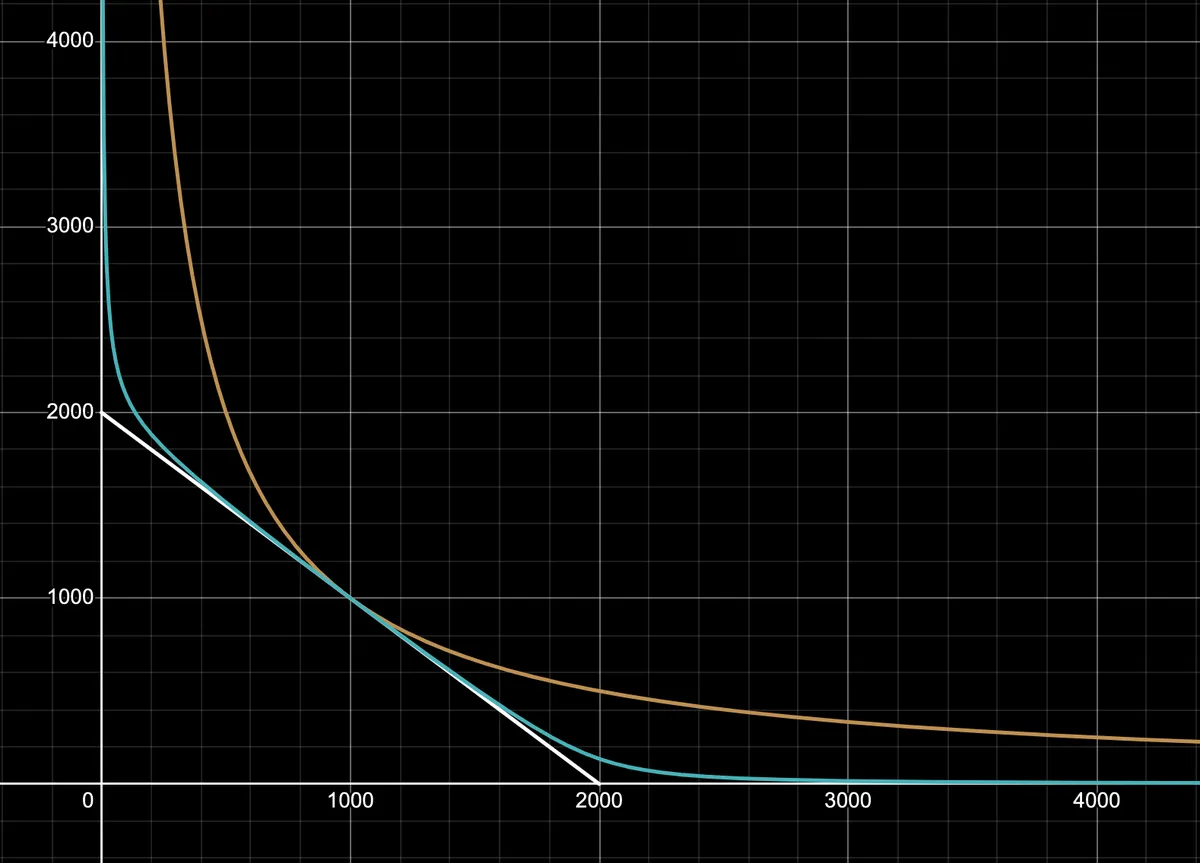
G.12: graph of the v4 invariant with $A=10$ and $D=2000$

Finally, the Curve invariant can be generalized for a pool of $n$ tokens instead of fixing $n=2$ as we have done in this post.

$\chi =\frac{A·{\prod }_{i=1}^n{x}_i}{{\left(\frac{D}{n}\right)}^n}$

$\chi ·D^{n-1}·{\sum }_{i=1}^n{x}_i+{\prod }_{i=1}^n{x}_i=\chi ·D^n+{\left(\frac{D}{n}\right)}^n$

Sources:

• Curve v1 whitepaper: https://resources.curve.fi/pdf/curve-stableswap.pdf
• This incredible blog on Curve math: https://alvarofeito.com/articles/curve/
• This incredible video course on Curve: https://updraft.cyfrin.io/courses/curve-v1